Edge Inference Benchmark Lab — FP32 vs FP16 vs INT8 on Jetson Orin Nano: What Do You Actually Gain?
Introduction
This article is adressed to fellow Edge AI enthusiasts, engineers and researchers.
This is the first part of my new Physical AI series focusing on efficient model deployment on edge devices. This will be a journey for me and hopefully for you, the reader, too. My goal through this series is to contribute with useful insights in an emergind domain and to give you some take away for your own projects, such as the approach, the hardware constraints, the architectural thinking, the data used, or the lessons learned along the way.
The main skills or prerequisites to this article and learning project are ONNX, TensorRT, quantization, CUDA ecosystem, roofline analysis, profiling, embedded deployment.
Note: all data you will read and see in the tables and on the graphs comes from my own measurements on my NVIDIA Jetson Orin Nano Developer Kit. If you want to learn more, dive deep into the code or even reproduce the results, I encourage you to check the repository on my GitHub account. All commands I used are documented in the summary.md files alongside the results. One warning before you try: if you are on an Orin Nano Developer Kit, verify your actual GPU clocks before anything else — the JetPack installer can cap the board at 15 W. See Hardware & Software below.
My goal with this project is not only to write a benchmark script and reason about a single model run, but also to develop a benchmark harness that is reusable in the future.
This article focuses on three measurements:
- Latency measurement: how much time we gain by reducing precision, with and without using CUDA Graph.
- Accuracy evaluation using the ImageNetV2 dataset
- Measuring power consumption at idle and during inference
Table of contents
- Introduction
- About the project setup
- Build pipeline
- FP32, TF32, FP16, INT8 Latency check
- Running the benchmark on a real dataset
- Power consumption
- Conclusion
- References
About the project setup
Model
In this article I am going to use the MobileNetV2 deep learning model from the ONNX model zoo [1].
MobileNet models perform image classification - they take images as input and classify the major object in the image into a set of pre-defined classes. They are trained on the ImageNet dataset, which contains images from 1000 classes. MobileNet models are also very efficient in terms of speed and size and hence are ideal for embedded and mobile applications, which makes it a good candidate model for the benchmark test on NVIDIA Jetson Orin Nano.
Its main characteristic is the depthwise separable convolution. A normal convolution would mix information across space and across channels in one operation, which is expensive. However, MobileNet splits that into two cheaper steps: a depthwise conv that filters each channel independently (spatial mixing only), then a pointwise 1×1 conv that combines channels (channel mixing only). Same expressive task, roughly 8–9× fewer multiplications [2].
Hardware & Software
If you’re not familiar with the Jetson Orin Nano, a few points worth mentioning:
- Compared to the Orin NX or AGX Orin, the Nano has no Deep Learning Accelerator (DLA), so we should deliberately avoid all DLA-based methodologies.
- Memory is unified: there is no PCIe ‘host <-> device’ copy, which means the GPU and the CPU address the same LPDDR5. As a result, the H2D and D2H are the same DRAM copy: it costs bandwidth but no bus transfer, and it can be bypassed entirely with pinned/mapped memory.
- The Tensor Cores on Ampere architecture support FP16, BF16, TF32, INT8, INT4 but not FP8, which is an important point for FP8 or NVFP4 quantization.
- The Ampere architecture supports 2:4 structured sparsity.
If you are using an NVIDIA Jetson Orin for the first time, make sure that you have the latest bootloder version on your device. After the first run of my computer I realised that Super Mode was not active and could not be activated. The JetPack 7.2 installer misdetected the Orin Nano Developer Kit and omitted the 25 W and MAXN SUPER power profiles, capping the board at 15 W / 624 MHz. I tried editing the nvpmodel config, symlinking the correct configuration files, but it did not help. Although nvpmodel -q showed 25 W, the actual clocks did not change, which makes me think that the clock ceilings come from the bootloader. In the end, a firmware update including installing the latest nvidia-l4t-bootloader version fixed the issue, moving L4T from 39.2.0 to 39.2.1 (R39 revision 2.0 to 2.1).
One easy way to verify it, part from using nvpmodel -q, always check what are the currently applied GPU clocks:
sudo jetson_clocks --show | grep -E 'GPU|EMC'
# For 25 W:, should be: GPU 918000000   EMC 3199000000
# For 15 W, capped profile: GPU 624000000
There is another way to notice it. The board reports a different model name once the firmware is right. Before the update it identified itself as NVIDIA Jetson Orin Nano Developer Kit; afterwards as NVIDIA Jetson Orin Nano Engineering Reference Developer Kit Super. Same board, same chassis, different string. Both captures are committed, check them out for comparison — before and after
For inference benchmarks there is a second reason for checking the board clocks. The board actively manages frequency based on the power mode (nvpmodel) and thermal state, optizing using a technique called dvfs (dynamic voltage and frequency scaling). It is a very useful technique to save energy during idle time, when the board is not under load. However, for latency benchmarking it can introduce extra latency increase, that we can eliminate by pinning the clock to the maximum using the following command:
sudo jetson_clocksTherefore, every single measurement row records the nvpmodel mode and whether jetson_clocks was applied. Later we will see its effect on power consumption and the throughput.
The benchmark included FP32, TF32, FP16 and INT8, where TF32 is a Tensor Core format with FP32 range and FP16-ish precision. By default TensorRT uses TF32 in an FP32 engine unless –noTF32 is passed. Making this distinction consciously is what stops us from reporting a TF32 run as the FP32 baseline.
Optimization task
In every optimization task, we have to think about what we are optimizing for and what our constraints are. Is it computation? Is it memory? Technically speaking, are we computation-bound or memory-bandwidth-bound? To come up with the right solutions or answers we have to identify the real bottleneck. During quantization we reduce the precision, which reduces the number of bytes we move, which in turn should reduce the latency. At least, that is our expectation.
What I expected
Before any tests, it can be interesting to make our own expections based on read literature, assumptions and engineeering judgement. It helps us later evaluate where we were right and where the measurements proofed us wrong.
1. The gains will track bytes, rather than arithmetic. MobileNetV2 is built from depthwise separable convolutions — cheap in multiplications, expensive in memory traffic per unit of work. If the network is memory-bound then we would expect that halving the element size should roughly halve the time, and the Tensor Core rate should be largely beside the point. So: expect around 2× from FP16, not the 8× its peak throughput suggests.
2. FP16 costs nothing measurable in accuracy, INT8 costs a little. This assumption is conventional for image classification, but since MobileNetV2 is a small model with little redundancy to spare.
3. CUDA Graph improves latency mosly where the kernels are shortest. It removes host-side launch overhead, which is a roughly fixed cost per kernel, so its benefit should grow as the per-kernel work shrinks: largest at INT8, smallest at FP32.
4. Lower power mode is more efficient. Dynamic power rises faster than linearly with clock, so a lower power mode should win on energy per frame even though each frame takes longer. Expect 15 W to beat 25 W on mJ/frame.
5. The derived ceilings are trustworthy. Peak compute comes from the Ampere SM rates [3], bandwidth from the bus width and memory clock. We can assume there is no reason to doubt arithmetic this simple.
Build pipeline
Let’s consider the following build pipeline:
  PyTorch nn.Module          ← source code (Python, eager, dynamic)
         │  torch.onnx.export / torch.export
         ▼
  ONNX graph (.onnx)         ← portable IR (static graph, typed tensors, opset-versioned)
         │  TensorRT builder  (optimising compiler + autotuner)
         ▼
  TensorRT engine (.plan)    ← target-specific binary (NOT portable)
         │  TensorRT runtime
         ▼
  CUDA kernels               ← the actual machine code, dispatched to SMs
         │
         ▼
  Ampere SMs + Tensor Cores  ← silicon
MobileNetV2 is available in an intermediate representation (IR) static graph format (.onnx extension) on Hugging Face. In the model used here, mobilenetv2-12.onnx, the 12 describes the opset version, which defines the semantics of operators such as Conv.
An ONNX graph contains:
- Nodes: operations such as
Conv,Add, andClip - Initializers: learned weights and biases stored as constants
To understand the architecture of the network we can use
polygraphy.
To make the model specific to the target hardware, I used trtexec to create the engine files (.plan) for the different data types: FP32, TF32, FP16 and INT8. I fixed the min, opt and max shape to 1x3x224x224 and added the –noTF32 flag to build the FP32 engine.
Tactic selection is stochastic in the tails. Two builds of the same ONNX on the same board can pick different tactics if the board was thermally different during the build. Rebuild determinism is a real methodological issue, this is why I took great care of the documentation in the repository, versioning and logging everything that matters.
Quantization for INT8
INT8 has 256 values to work with, so every tensor needs a scale: a number mapping its floating-point range onto that grid. Weights are known when you build, so their ranges are too. Activations are not — they depend on the input — so they have to be measured. That measurement is calibration: push a sample of real images through the network and record how large each activation actually gets.
I used 512 images from the calibration split, stratified across all 1000 classes and disjoint from the evaluation set, preprocessed through the same code path evaluation uses. Both constraints matter. Calibrating on evaluation images leaks the test set into the model. Calibrating with different preprocessing — a different resize, say — measures activation ranges the deployed model never sees.
For choosing where to clip I used the entropy method rather than max. Max takes the largest value observed, which one outlier can stretch, wasting most of the 256 levels on a range nothing occupies. Entropy picks the clip point that loses the least information, accepting that a few extremes saturate.
python scripts/quantize_int8.py --n 512 --method entropy
scripts/quantize_int8.py— calibration set selection, the ModelOpt [5] call and the node census it prints afterwards.
The output is an ONNX file, with QuantizeLinear/DequantizeLinear pairs inserted that carry the scales. This is called explicit path: the scales live in the graph, so TensorRT has no discretion about which layers run in INT8. The older approach called implicit path (a calibrator handed to the builder, deprecated since TensorRT 10.1 [4]) lets TensorRT quietly keep layers in FP16 where that is faster — sensible when shipping, useless for a benchmark whose whole question is what actually executed.
After quantization:
| Before | After | |
|---|---|---|
| Nodes | 105 | 318 |
| Q/DQ pairs | 0 | 105 |
| Conv | 52 | 52 |
| “Quantized” nodes | — | 64 |
Each quantized tensor gets a QuantizeLinear + DequantizeLinear pair, so 105 pairs = 210 extra nodes. These are not extra work at runtime — TensorRT reads them as precision annotations and folds them into the kernels. The graph gets bigger; the engine shouldn’t. There are 105 Q/DQ pairs, but only 64 nodes are considered “quantized”.
FP32, TF32, FP16, INT8 Latency check
To measure only inference latency we measure how fast the model performs without any pre-processing or post-processing steps. At this point we don’t use real photos, only memory garbage to see how fast the neural network performs from the input layer to the output layer.
For each run we:
- Fix the min, opt and max shape to: 1x3x224x224
- Define 2000 ms warmup
- Run the inference for 30 seconds
- Pin GPU clock to max
Performance summary without CUDA Graph
Source:
results/run/20260919T211117Z_7eb0b09/summary.mdfor FP32/TF32/FP16 andresults/run/20260920T102737Z_bff3273/summary.mdfor INT8. Both carry the build and benchmark commands, the raw trtexec logs and the per-layer exports.
| Metric | FP32 | TF32 | FP16 | INT8 | INT8 / FP32 |
|---|---|---|---|---|---|
| Throughput (qps) | 518.057 | 671.866 | 1047.750 | 1309.840 | 2.528x |
| Median latency (ms) | 1.9805 | 1.5342 | 0.9902 | 0.8086 | 0.408x |
| Latency p99 (ms) | 1.9895 | 1.5430 | 1.0061 | 0.8164 | 0.410x |
| GPU compute median (ms) | 1.9277 | 1.4844 | 0.9439 | 0.7607 | 0.395x |
| Enqueue median (ms) | 0.5459 | 0.5264 | 0.5830 | 0.5371 | 0.984x |
| Enqueue / compute ratio | 0.2833 | 0.3545 | 0.6177 | 0.7060 | 2.493x |
| Throughput speedup vs. FP32 | 1.000x | 1.297x | 2.022x | 2.528x | — |
| Latency speedup vs. FP32 | 1.000x | 1.291x | 2.000x | 2.449x | — |
Performance summary with CUDA Graph
| Metric | FP32 | TF32 | FP16 | INT8 | INT8 / FP32 |
|---|---|---|---|---|---|
| Throughput (qps) | 573.177 | 777.122 | 1327.200 | 1711.850 | 2.987x |
| Median latency (ms) | 1.7930 | 1.3320 | 0.7949 | 0.6260 | 0.349x |
| Latency p99 (ms) | 1.8027 | 1.3408 | 0.8123 | 0.6328 | 0.351x |
| GPU compute median (ms) | 1.7402 | 1.2832 | 0.7490 | 0.5820 | 0.334x |
| Enqueue median (ms) | 0.0254 | 0.0098 | 0.0098 | 0.0078 | 0.308x |
| Enqueue / compute ratio | 0.0146 | 0.0076 | 0.0130 | 0.0134 | 0.920x |
| Throughput speedup vs. FP32 | 1.000x | 1.356x | 2.316x | 2.987x | — |
| Latency speedup vs. FP32 | 1.000x | 1.346x | 2.256x | 2.864x | — |
- FP16 remains effectively free from an accuracy perspective while significantly improving latency and throughput.
- INT8 keeps high performance with a small accuracy loss, around 0.78 points of Top-1 on this dataset.
- CUDA Graph reduces the host-side overhead substantially in the INT8 run, improving the median latency from about 0.809 ms to about 0.626 ms.
- Throughput speedup exceeds latency speedup, and the gap widens as the kernels get shorter: trtexec overlaps the H2D and D2H copies with compute across iterations, so the roughly 0.04 ms of transfer per query is hidden. That overhead is a larger share of a 0.58 ms INT8 kernel than of a 1.74 ms FP32 one, which is why INT8 reaches 2.987x on throughput but 2.864x on median latency, while TF32 shows almost no divergence (1.356x vs 1.346x).
- The current run confirms the expected pattern: the INT8 graph-enabled configuration is the fastest measured variant in this benchmark set.
FP16 has 8× the peak of true FP32. We got 2.02×. And it’s not a coincidental 2× — it’s the bandwidth ratio. FP16 halves every byte moved, and the network is memory-bound, so the gain tracks the bytes rather than the flops.
Compare the two steps directly:
FP32 → TF32: 4× more compute, same bytes → 1.29× TF32 → FP16: 2× more compute, half the bytes → 1.56×
More compute alone bought us 29%. Half the data bought us 56% on top of a smaller compute bump. On this board, bytes are worth more than flops.
Learned after running CUDA Graph:
The enqueue median dropped from 0.5371 ms to 0.0078 ms, which is a ~69× reduction for INT8. The CUDA Graph hypothesis is confirmed. The enqueue collapse is expected — one graph launch replaces 57 individual ones.
But GPU compute also dropped 23%, and that shouldn’t happen. The kernels are identical; same engine file, no rebuild. What changed is that without a graph, the CPU issues each launch individually, and small kernels finish faster than the CPU can queue the next one. The GPU sits idle in the gaps, and those gaps land inside the measured GPU time. CUDA Graphs pre-stage the whole sequence so kernels dispatch back-to-back.
So that 0.179 ms wasn’t compute at all — it was launch latency bubbles between 57 short kernels. CUDA Graphs bought us 1.26×, comparable to the entire FP32→TF32 precision step. A free flag, no accuracy cost, no rebuild: the cheapest speedup on this board isn’t a precision change.
In a pure inference setting, where everything is static — fixed shapes, fixed buffers — CUDA Graph brought an instant benefit. In a real pipeline, though, where camera capture, resize and normalise come first and NMS or argmax come after, we only speed up the inference stage, which is a fraction of the whole pipeline. There, the integration is the real work.
Does --useSpinWait add anything?
--useSpinWait changes only how the host waits for the GPU to finish: it busy-polls instead of blocking on an event. I ran it on top of CUDA Graph, for TF32 only.
| Metric | TF32 graph | + spinWait | Δ |
|---|---|---|---|
| Throughput (qps) | 777.122 | 777.626 | +0.06% |
| Median latency (ms) | 1.33203 | 1.32520 | −0.5% |
| Latency p99 (ms) | 1.34082 | 1.33398 | −0.5% |
| GPU compute median (ms) | 1.28320 | 1.28320 | 0 |
| Enqueue median (ms) | 0.009766 | 0.006348 | −35% |
The GPU compute median is bit-identical, which is exactly what should happen: spinWait touches the host side only. The 35% cut in enqueue is real, but it recovers 3.4 µs against a 1.28 ms kernel, so end to end it disappears into run-to-run noise.
The reason is that CUDA Graph has already removed the launch overhead that spinWait would otherwise hide. Both flags attack the same bottleneck, so they do not compose. And unlike a graph, this one is not free on an edge device: busy-polling burns a CPU core for no measurable latency gain, which is a bad trade on a board where the metric that matters is mJ per frame.
Running the benchmark on a real dataset
In this chapter I’m using the ImageNetV2 matched-frequency set [6], [7].
It contains 10,000 images across 1000 classes, a 1000-image calibration set, 9000 for eval and no overlap between those two. I deliberately used PIL instead of OpenCV during the preprocessing, because the two produce different pixel values for the same resize, and torchvision’s reference accuracy came from the PIL path. Mixing them might manufacture a 1-2% “quantization loss” that is really just a resize bug. The results include a fingerprint for the split to prove that two runs used the same images. The split is also saved in a json file with the fingerprint, so it is traceable in the repository.
One notes: ImageNetV2 was built to be harder than the original validation set, so the expectation for ImageNetV2 is lower than for the ImageNet validation set. It lands at around 58–61% instead of 71.9% [8].
The FP32 accuracy baseline
I ran the FP32 accuracy baseline test first through ONNX Runtime on CPU, not TensorRT. ORT is an independent implementation, so if the result matches my TensorRT FP32 engine later, then that is proof that my engine is correct.
One methodological lesson I learned: To test my eval script I ran only the first 500 images instead of the whole dataset, then ran it on all 9000 images, printing the results after every 500 images. Surprisingly, the Top-1 and Top-5 accuracies were consistently dropping over time. Aftet inspecting the data, I realised that the data is sorted by class index and that the first 100 images contain only animal classes, where the model performs better. So it is a biased subset. I could easily eliminate this bias with a random shuffle step during the preprocessing phase. So if you see similar behaviour during testing, this is one thing you can suspect.
So the results:
The same test run on TensorRT gave an identical result, so the baseline is locked to:
| Backend | Top-1 | Top-5 |
|---|---|---|
| ONNX Runtime CPU FP32 | 58.61% ± 1.02% | 81.11% |
| TensorRT FP32 | 58.61% ± 1.02% | 81.11% |
FP32, TF32, FP16, INT8 accuracy
Source:
results/run/20260920T102737Z_bff3273/summary.md. The evaluation split is pinned by fingerprint indata/split_v1.json, so the same 9000 images back every row.
| Precision | Top-1 | Top-5 | Top-1 Δ vs. FP32 |
|---|---|---|---|
| FP32 | 58.61% | 81.11% | — |
| TF32 | 58.57% | 81.08% | -0.04 pts |
| FP16 | 58.59% | 81.04% | -0.02 pts |
| INT8 | 57.83% | 80.47% | -0.78 pts |
The conclusion: FP16 costs nothing measurable in accuracy and delivers 2.32× the throughput. There is no reason to deploy FP32 on this board.
The engine nearly halved: 14.40 → 7.35 MB, a factor of 1.96×. Device memory halved exactly: 7.02 → 3.51 MB (7,024,640 → 3,512,320 bytes). The memory halved precisely while latency improved only 2.26× against a theoretical 8×.
As we lower precision, we capture a smaller share of the theoretical gain — 34%, 29%, 19%. The hardware’s arithmetic ceiling rises 16× while the delivered speedup rises 2.99×, because the bottleneck was never arithmetic.
FP16→INT8 graphed is 1.29×, close to the 1.25× we saw ungraphed. Consistent across two measurement methods.
Roofline Analysis
So far the argument has been circumstantial. FP16 delivered 2.02× against a theoretical 8×, the gain tracked the bytes rather than the flops, and from that I inferred the network is memory-bound. A roofline turns the inference into a measurement: put every layer on a plot of arithmetic intensity against attained throughput, draw the two ceilings the hardware imposes, and see which one each layer is actually up against.
How these numbers were produced
Source:
results/profiles/summary-276801ac2b6a.md, ten runs across four precisions. The measurement isscripts/profile_model.py; the FLOP and byte accounting, including the grouped-convolution and fusion handling described below, isframecost/roofline.py.
scripts/profile_model.py invokes trtexec once with --dumpProfile --separateProfileRun. That yields a per-layer table from an instrumented pass and a clean Performance summary from an uninstrumented one, in the same process — so there is no thermal drift between two commands. Per-layer times are then scaled so their sum matches the clean GPU compute time. That correction is 5.6% at FP32 and 24.2% at INT8: the profiling hooks cost a fixed amount per layer, and the kernels get shorter as precision drops.
Layer geometry comes from the ONNX graph, which matters more than it sounds. MobileNetV2’s depthwise convolutions have groups == C_in; ignoring the group attribute overstates their FLOPs by up to 32× and moves them to the wrong side of the ridge. A fused TensorRT layer such as Conv_5 + Clip_6 ran as one kernel, so the intermediate never reaches DRAM — the group is charged the first node’s input, the last node’s output and all its weights, not the sum of each node’s traffic. Reformat and quantise nodes are excluded from FLOP attribution entirely.
Clocks are read from tegrastats during the run, every run below measured 904–907 MHz against a nominal 918 MHz at 25 W.
The peak ratios (TF32 4×, FP16 8×, INT8 16× vs FP32) come from the Ampere SM rates: 256 FLOP/SM/clk on the CUDA cores for FP32, against 1024 / 2048 / 4096 on the Tensor Cores. They check out against the board spec — 4096 × 8 SM × 1020 MHz is 33.4 TOPS dense, i.e. the advertised 67 TOPS sparse [9] — and against the 40 TOPS quoted for the original 625 MHz Orin Nano.
Measuring the ceiling instead of deriving it
Source:
results/peak_gemm/summary-a74615cea83b.md, measured byscripts/peak_gemm.py.
One of those ratios could have been wrong by a factor of two, and it is the one the whole chapter leans on. Consumer Ampere halves FP16 throughput when accumulating in FP32 — an RTX 3080 does 119 TFLOP/s with FP16 accumulate and 59.5 with FP32 [3] — while the datacenter A100 has no such penalty. Orin is neither. If its GA10B inherits the GeForce behaviour, the FP16 ceiling is 7.5 TFLOP/s rather than 15.0, the ridge is 72 rather than 145, and every FP16 percentage above is out by 2×.
A datasheet cannot settle this, so I measured it. A large square matmul is deeply compute-bound — the opposite regime from MobileNetV2 — so what it attains is limited by arithmetic and nothing else. FP32 serves as the control: it runs on the CUDA cores with no Tensor Core and no accumulate ambiguity, so if it lands near its own ceiling the harness is sound.
| Precision | Ceiling | Attained | % of ceiling |
|---|---|---|---|
| FP32 (control) | 1.88 T/s | 1.50 | 79.6% |
| TF32 | 7.52 T/s | 4.01 | 53.3% |
| FP16 | 15.04 T/s | 9.97 | 66.3% |
The halved FP16 ceiling would be 7.52 T/s. FP16 reached 9.97, exceeding it by a third. A roof cannot be beaten, so the penalty does not apply.
The test is deliberately one-sided. Any inefficiency in the harness — a poor tactic, a thermal dip, a kernel that never saturates — pushes attained throughput down, so “closer to 7.5 than to 15.0” could be manufactured by a bad measurement. Exceeding 7.5 cannot be. Only the affirmative direction proves anything, which is why falling short would have been reported as inconclusive rather than as evidence of a penalty.
Strictly, what this shows is that FP16 with FP16 accumulate is not halved, since that is the kernel TensorRT chose — sm80_xmma_gemm_f16f16_f16f16_f16_..., where the trailing f16 is the accumulator. Which would leave the question open, except that MobileNetV2’s own engine turns out to use the same mode: its convolutions compile to sm80_xmma_fprop_implicit_gemm_f16f16_f16f16_f16_.... So the measured ceiling is the right one for the engine on the plot, whatever Orin does with FP32 accumulate elsewhere.
The habit worth taking from this: a derived ceiling is a hypothesis. This one held, but it was one plausible hardware detail away from putting every FP16 point on this roofline in the wrong place.
The ceilings, and where the model sits
| FP32 | TF32 | FP16 | INT8 | |
|---|---|---|---|---|
| Peak compute (T/s) | 1.85 | 7.41 | 14.82 | 29.71 |
| Ridge (FLOP/byte) | 18.1 | 72.4 | 144.8 | 290.2 |
| AI median (FLOP/byte) | 13.24 | 13.24 | 26.47 | 52.95 |
| Memory-bound layers | 36 / 52 | 52 / 52 | 52 / 52 | 52 / 52 |
| GPU compute (ms) | 1.920 | 1.483 | 0.938 | 0.759 |
| Achieved BW, median (GB/s) | 28.9 | 38.3 | 29.7 | 17.6 |
| — as share of bandwidth peak | 28% | 37% | 29% | 17% |
| — as share of compute peak | 20% | 8% | 6% | 3% |
Memory bandwidth is fixed at 102.4 GB/s throughout — LPDDR5 at 3199 MHz over a 128-bit bus, double data rate.
The last two rows are the same layers measured against the two different ceilings, and they disagree. Against the compute roof, utilisation falls steadily as precision drops — which says nothing useful, because none of these layers is anywhere near that roof. Against the memory roof it peaks in the middle. TF32 reaching 37% of the bandwidth ceiling while sitting at 8% of the compute ceiling is the whole argument of this section in two numbers.
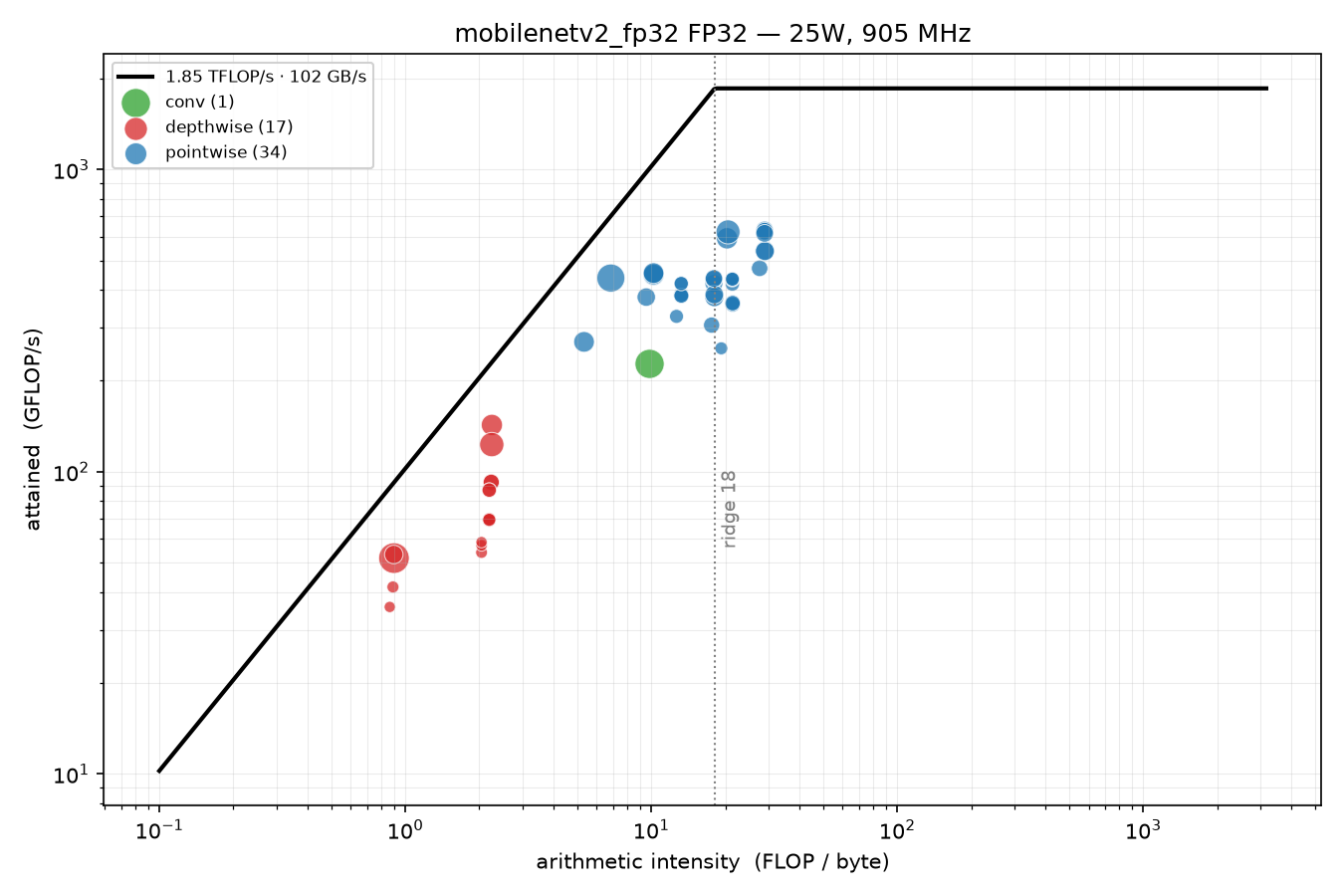
FP32. Ridge at 18 FLOP/byte. The pointwise cluster straddles it — sixteen layers sit to the right, where arithmetic is the binding constraint. Run 20260925T195311Z.
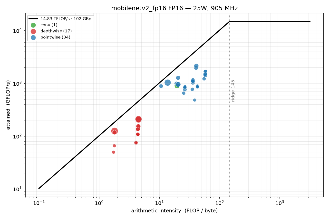
FP16. Same network, same 905 MHz, but the roof is 8× higher so the ridge has moved to 145 — far beyond the rightmost layer at 58. Nothing is compute-bound any more, and the gap never closes again at INT8. Run 20260925T172315Z.
Point area is share of runtime; colour is layer kind. Both figures come from ungraphed runs — the CUDA Graph run’s per-layer throughput is inflated by its scale factor and is not usable here. The TF32 and INT8 plots are in the repository and tell the same story as FP16.
Worth reading the vertical position as well as the horizontal. A point sitting on the diagonal is saturating memory bandwidth; a point below it is achieving neither ceiling. In FP32 the depthwise cluster at AI ≈ 1 attains about 50 GFLOP/s where the memory roof allows 92 — roughly half. In FP16 the layers around AI 10–20 hug the diagonal, while those out at AI 30–60 fall well below it. Those lower points are the layers too small to saturate anything, and they are the reason a launch-overhead fix like CUDA Graph could buy 1.26× on a workload that is nominally bandwidth-limited.
FP32 is the only precision with compute-bound layers. Its roof sits at 1.85 TFLOP/s, the CUDA cores alone, so the ridge falls at just 18.1 FLOP/byte and sixteen layers sit above it. All sixteen are pointwise convolutions, and they carry 44% of the model’s arithmetic in 27% of its runtime.
Engage the Tensor Cores and that disappears. TF32 lifts the roof 4×, the ridge moves to 72.4, and every layer drops to the memory-bound side. It never comes back: FP16 and INT8 push the ridge to 144.8 and 290.2 while the workload’s intensity rises only in step with it. The most arithmetic-intense layer in the network reaches 40% of the ridge in FP16 and 40% in INT8 — the same relative position, because halving the element size doubles the intensity and doubles the ceiling at once.
This explains the whole precision sweep
| Step | Measured | Theoretical | Captured |
|---|---|---|---|
| FP32 → TF32 | 1.296× | 4× | 32.4% |
| TF32 → FP16 | 1.581× | 2× | — |
| FP16 → INT8 | 1.236× | 2× | — |
| FP32 → INT8 | 2.533× | 16× | 15.8% |
FP32 → TF32 buys 1.296× because roughly a third of the layers genuinely were arithmetic-limited. That is the one step in this sweep where more FLOP/s is the right medicine, and the roofline says exactly why: those sixteen pointwise convs were sitting on the compute roof.
Every step after it is pure byte reduction. TF32 → FP16 and FP16 → INT8 track the halving of traffic, not the doubling of arithmetic they nominally offer. Which is the earlier claim — bytes are worth more than flops on this board — now with a precise boundary on it. Flops mattered exactly once, at the CUDA-core-to-Tensor-Core transition, and never again.
These GPU-compute figures come from a different measurement path than the latency chapter (per-layer profiling with --noDataTransfers, against end-to-end throughput) and land on the same ratios: 1.296 against 1.297 for FP32 → TF32, and 2.533 against 2.528 for FP32 → INT8. Two independent methods, three decimal places.
Memory-bound, but not bandwidth-saturated
There is a second finding hiding behind the first. Achieved bandwidth is not monotonic: 28.9 → 38.3 → 29.7 → 17.6 GB/s. It peaks at TF32 and falls away.
The best layers do saturate the bus — 81% of peak in FP16, 74% in INT8. The median layer reaches under a third. So the typical layer is limited by neither ceiling on the plot; it is simply too small to saturate anything, and what bounds it is launch latency and occupancy. Each precision step halves the bytes but shrinks the kernels, and shorter kernels use the bus worse, so you never collect the full 2× that halving the traffic promises.
That reframes the CUDA Graph result rather than contradicting it. A genuinely bandwidth-saturated GPU could not gain 1.26× from removing launch overhead. The fact that it did is this same finding seen from the other side, and the distinction matters practically: “memory-bound” says quantise, “launch-bound” says fuse and batch.
Even the FP32 layers that are compute-bound only reach 25–34% of their 1.85 T/s roof. Above the ridge does not mean saturating the ALUs; it means the memory ceiling is no longer the binding one.
What the depthwise convolutions cost
| Kind | n | Share of FLOPs | Share of time | Cost per FLOP |
|---|---|---|---|---|
| depthwise | 17 | 6.9% | 32.2% | 4.7× |
| pointwise | 34 | 89.1% | 51.2% | 0.57× |
Depthwise convolutions are eight times more expensive per FLOP than pointwise ones, and they hold the lowest arithmetic intensity in the network (1.73 for Conv_7 + Clip_8). The depthwise separable convolution buys MobileNet an 8–9× reduction in multiplications and hands roughly a third of it straight back in memory traffic. A FLOP count is not a runtime prediction.
One more line worth knowing: Reformatting CopyNode for Input Tensor 0 is the single largest non-compute item in the FP16 engine at 8.5% of profiled time, and CUDA Graph removes three quarters of it — 93.2 µs down to 27.2 µs. Part of that 1.26× the graph bought is not launch overhead in the abstract; it is this one node.
Reproducibility
Ten profile runs, four precisions, all pinned at 25 W. Repeated configurations agree to 0.07–0.32% on benchmark GPU time. Across the three FP16 repeats, per-layer times vary by a median of 1.1%, a p90 of 4.6% and a worst case of 8.4% — and that worst case is a 6 µs cast where half a microsecond of jitter is 8%. Arithmetic intensity, FLOP and byte counts are bit-identical across repeats, as they must be: they come from the graph, not the clock.
One caveat on the table above. The exact doubling of arithmetic intensity at each precision step is partly the model’s assumption rather than a measurement — ELEM_BYTES applies one element size to every tensor in an engine, so halving it mechanically doubles every AI. Real INT8 engines keep their quantise boundaries in wider types, visible here as a 55 µs input_QuantizeLinear. The direction of the finding is measured; the exactness is assumed.
Power consumption
In the previous chapter we could observe the trade-off between latency, throughput and accuracy. Discussing only quality and speed trade-offs assumes that energy is available without any limits. However, as soon as we run devices on battery with limited energy resources, we introduce a new variable called power, measured in watts. This brings us to the next measurements.
The sampler is framecost/telemetry.py and the measurement script is scripts/measure_energy.py.
NVIDIA Jetson Orin Nano is equipped with many sensors that can be read out in real time by running the built-in tegrastats function. It captures a lot of useful telemetry: instantaneous temperature, power, EMC and GPU frequency, used and available RAM. From this data, we can calculate mean and maximum values, energy per frame, as well as behaviour at idle and during inference.
In addition to the onboard measurement, I installed a power meter between the Jetson and the socket. This gives the total power that the Jetson consumes from the grid (or would do from a battery).
I used the WM03-DE model from Ningbo with the following parameters:
- EU type: Imax = 16A, Vn= 230V ~, P_max = 3680W
- Power display range: 0.5W-3680W
- Power Accuracy: ±2%
P_board is what VDD_IN measures: the DC input to the devkit after the barrel jack, sensed by the carrier-board INA3221, so it covers module and carrier loads. P_wall is what the WM03-DE measures at the socket, including PSU loss.
A note on the naming: tegrastats labels that channel VDD_IN, which names the rail rather than the quantity flowing on it. Since every number in these tables is a power in watts, I call it P_board and keep VDD_IN for the raw field in the code and the result files.
The decisive factor is the energy per frame, which we can call efficiency. It is calculated as follows:
$$ \text{mJ_per_inference} = \frac{\text{mean_power_W} \times \text{sampler_duration_s}}{\text{n_inferences}} \times 1000 $$
n_inferences differs per run, since the throughput is different for each precision. For example for INT8 at 25 W: 9.754 W × 123.5 s = 1204.6 J, divided by 184,488 = 6.53 mJ.
Repo reference: all results are documented in result.json, and the calculation is made by telemetry.py, which is called by measure_energy.py, the script used for the following measurements. The results are automatically saved with the following naming convention:
<timestamp_in_ISO_form>_<model>_<precision>_<power_mode>_<dvfs|pinned>_<last_short_commit_hash>
Efficiency with pinned vs unpinned GPU clock
Before benchmarking the models, it is worth measuring what difference it makes to pin the GPU clock to maximum versus using the built-in DVFS (dynamic voltage and frequency scaling) setting.
Unpinned vs. pinned
| Metric | Unpinned | Pinned | Δ |
|---|---|---|---|
| Throughput | 1320.0 qps | 1329.5 qps | +0.7% |
| P_board load | 13.797 W | 14.001 W | +1.5% |
| Total mJ/frame | 10.753 | 10.788 | +0.3% |
| P_board idle | 3.534 W | 5.827 W | +65% |
| P_wall idle | 5.25 W | 8.15 W | +55% |
P_wall / P_board ratio
| Metric | P_board | P_wall | Gap | Ratio |
|---|---|---|---|---|
| Idle unpinned | 3.53 W | 5.25 W | 1.72 W | 1.49× |
| Idle pinned | 5.83 W | 8.15 W | 2.32 W | 1.40× |
| Load unpinned | 13.80 W | 17.75 W | 3.95 W | 1.29× |
| Load pinned | 14.00 W | 17.95 W | 3.95 W | 1.28× |
The results show that pinning clocks costs 2.29 W at idle and buys only 0.7% throughput. Under continuous load it’s 0.7% more work for 1.5% more power, so energy per frame is marginally worse pinned. The entire cost lands at idle, and the wall meter confirms it independently: 2.9 W at the socket for a board doing nothing. That means 13.8 mJ/frame at the wall, against 10.8 mJ/frame from tegrastats.
Efficiency with FP16 and INT8 for different power modes
Source:
results/energy/summary-6fc2633c8be2.md, six runs.
As we concluded in the previous section, the DVFS version is more efficient, so all six of the following runs were executed with DVFS on. All six started at 46–47 °C, with idle baselines within 1% of each other.
FP16
| Mode | GPU max | Throughput | P_board | P_wall | Gap | mJ/frame (P_board) | mJ/frame (P_wall) | Tj max |
|---|---|---|---|---|---|---|---|---|
| 15 W | 612 MHz | 889.8 qps | 8.76 W | 11.65 W | 2.89 W | 10.10 | 13.43 | 54.7 °C |
| 25 W | 918 MHz | 1320.0 qps | 13.80 W | 17.75 W | 3.95 W | 10.75 | 13.83 | 61.5 °C |
| MAXN_SUPER | 1020 MHz | 1439.2 qps | 15.31 W | 19.70 W | 4.39 W | 10.90 | 14.02 | 63.3 °C |
| Idle | — | — | 3.52 W | 5.25 W | 1.73 W | — | — | 46.5 °C |
INT8
| Mode | GPU max | Throughput | P_board | P_wall | Gap | mJ/frame (P_board) | mJ/frame (P_wall) | Tj max |
|---|---|---|---|---|---|---|---|---|
| 15 W | 612 MHz | 1141.7 qps | 7.49 W | 10.15 W | 2.66 W | 6.73 | 9.11 | 52.9 °C |
| 25 W | 918 MHz | 1537.4 qps | 9.75 W | 12.95 W | 3.20 W | 6.53 | 8.67 | 56.7 °C |
| MAXN_SUPER | 1020 MHz | 1662.8 qps | 10.68 W | 13.95 W | 3.27 W | 6.58 | 8.60 | 57.8 °C |
Interpretation
- FP16 behaves as predicted — 15 W is the most efficient: 62% of MAXN’s throughput for 57% of the power, giving 7.3% better energy per frame. Slower is more efficient.
- INT8 inverts it: 25 W is the optimum on P_board, and MAXN_SUPER at the wall. 15 W is the worst of the three. That’s the opposite of the FP16 ordering. The difference between 25 W and MAXN_SUPER is very small, under 1%, which can be inside noise. But the direction of the shift is systematic, because the fixed 1.73 W is paid per second and so it penalises slower configurations.
- The reason is that at 15 W the GPU is capped at 612 MHz, but the 3.5 W static baseline is still paid for every frame and INT8 frames take 0.88 ms instead of 0.65 ms. By slowing down, the static share of each frame’s energy grows. FP16 is dynamic-power-dominated so lowering clocks wins; INT8 already cut dynamic power by 39%, so static overhead now dominates and stretching the frame costs more than the clock reduction saves.
- The practical statement: the optimal power mode depends on the precision you deploy.
One number for scale. Every figure above is inference, and inference is not what this board finds hard. Profiling a dense 2048² matmul — arithmetic-bound, nothing like a convolution network — drew 21 W sustained in the same 25 W mode where MobileNetV2 FP16 draws 13.8 W, with Tj at 65 °C and the GPU clock never dipping below 903 MHz of its 918 MHz ceiling. No throttling at either load. So the inference workload is running at roughly two thirds of what the board will actually pull, and the thermal and current headroom that matters for a sealed enclosure or a sustained duty cycle is larger than the inference numbers alone suggest.
Conclusion
What held and what did not
| Expected | Outcome |
|---|---|
| 1. Gains track bytes, not arithmetic | Held. 2.05× from FP16 against a theoretical 8×, and the roofline later showed why: all 52 layers sit left of the ridge. |
| 2. FP16 free, INT8 slightly costly | Held. −0.02 points Top-1 for FP16, −0.78 for INT8. |
| 3. CUDA Graph helps most at short kernels | Held, and then some. Enqueue collapsed 69×. But GPU compute dropped 23% too, which should not happen — kernels do not run faster because of how they were launched. |
| 4. Slower is more efficient | Held for FP16, inverted for INT8. 15 W is the most efficient mode for FP16; 25 W for INT8. |
| 5. The derived ceilings are trustworthy | Not safe to assume. The FP16 ceiling turned on whether Orin penalises FP32 accumulation — a factor of two — and had to be measured. |
The CUDA Graph compute drop resolved once the per-layer profile existed: without a graph the CPU cannot queue short kernels fast enough, the GPU idles in the gaps, and those gaps land inside the measured GPU time. It was never compute; it was 0.179 ms of launch bubbles between 57 kernels.
The INT8 inversion is the finding I would keep if I could keep only one. At 15 W the GPU is capped at 612 MHz, but the 3.5 W static baseline is paid per second regardless, and INT8 frames take 0.88 ms instead of 0.65 ms. FP16 is dynamic-power-dominated, so lowering the clock wins. INT8 has already cut dynamic power by 39%, so the static share dominates and stretching the frame costs more than the slower clock saves. The optimal power mode is not a property of the board. It is a property of the board and the precision together.
The ceiling that needed measuring is the methodological one. A derived number that everything else divides by is a hypothesis wearing the clothes of a constant.
Three things I did not predict at all
The board did not have the performance modes it was sold with. The JetPack installer misdetected the devkit and omitted the 25 W and MAXN SUPER profiles, capping it at 624 MHz while nvpmodel cheerfully reported 25 W. Every number here would have been roughly half, with nothing obviously wrong.
“Memory-bound” turned out to understate it. The roofline says every layer is bandwidth-limited, but achieved bandwidth says the median layer reaches under a third of the bus. Most layers are too small to saturate anything; what bounds them is launch latency and occupancy. That is why a launch-overhead fix bought 1.26×.
Depthwise convolutions cost 8× more per FLOP than pointwise ones. They carry 6.9% of the arithmetic and 32% of the runtime. The operation that makes MobileNet cheap in multiplications hands roughly a third of that saving straight back as memory traffic.
The shape of the thing
NVIDIA sells this board as 67 TOPS. Dense, that is 33.4. At 918 MHz the arithmetic ceiling is 15.0 TFLOP/s in FP16, and the best layer in this network attained 2.1. The gap between the number on the box and the number on the board is not a defect in either — it is the entire subject. Every technique in this article, precision reduction included, is an attempt to close a little of it, and the roofline is what tells you which attempts can possibly work.
For MobileNetV2 on an Orin Nano the answer was: bytes, not flops, and only once — the step onto the Tensor Cores. Everything after that was traffic. A different network, with different arithmetic intensity, will give a different answer, which is why the harness matters more than these particular numbers.
References
External sources only. Everything measured in this article links inline to the artifact in the repository that produced it.
[1] ONNX model zoo, mobilenetv2-12. https://huggingface.co/onnxmodelzoo/mobilenetv2-12
[2] M. Sandler, A. Howard, M. Zhu, A. Zhmoginov, L.-C. Chen. MobileNetV2: Inverted Residuals and Linear Bottlenecks. CVPR 2018. arXiv:1801.04381. https://arxiv.org/abs/1801.04381
[3] NVIDIA. NVIDIA Ampere GA102 GPU Architecture whitepaper, v2.1. https://www.nvidia.com/content/PDF/nvidia-ampere-ga-102-gpu-architecture-whitepaper-v2.1.pdf — SM composition (128 CUDA cores, four third-generation Tensor Cores) and the GeForce FP16-with-FP32-accumulate rate.
[4] NVIDIA. TensorRT 10.1.0 Release Notes. https://docs.nvidia.com/deeplearning/tensorrt/10.x.x/getting-started/release-notes-10/10.1.0.html — deprecates the INT8 implicit quantization and calibrator APIs, IInt8EntropyCalibrator2 among them, recommending explicit quantization instead.
[5] NVIDIA Model Optimizer, ONNX quantization guide. https://nvidia.github.io/Model-Optimizer/guides/_onnx_quantization.html (repository: https://github.com/NVIDIA/Model-Optimizer, formerly TensorRT-Model-Optimizer)
[6] B. Recht, R. Roelofs, L. Schmidt, V. Shankar. Do ImageNet Classifiers Generalize to ImageNet? ICML 2019. arXiv:1902.10811. https://arxiv.org/abs/1902.10811
[7] ImageNetV2 matched-frequency set. https://huggingface.co/datasets/vaishaal/ImageNetV2/resolve/main/imagenetv2-matched-frequency.tar.gz
[8] torchvision, mobilenet_v2 — MobileNet_V2_Weights.IMAGENET1K_V1, 71.878% top-1 / 90.286% top-5 on ImageNet-1K. https://docs.pytorch.org/vision/main/models/generated/torchvision.models.mobilenet_v2.html
[9] NVIDIA. Jetson Orin Nano Super Developer Kit. https://www.nvidia.com/en-us/autonomous-machines/embedded-systems/jetson-orin/nano-super-developer-kit/ — 67 sparse TOPS, 102 GB/s, 1024 CUDA cores and 32 Tensor Cores, 7–25 W; and the 40 TOPS / 68 GB/s figures for the pre-Super configuration.